

The CLS Forecasting Benchmark on the 15-Minute Market
With the same inputs and the same decision time, the forecasting function of our Continual Learning System (CLS) earned more simulated battery revenue than TabPFN 2.5 over the first year of 15-minute trading on the German-Luxembourg day-ahead market: 91.4% of the perfect-foresight maximum against 89.8%, +433 EUR per day (95% interval +159 to +710), while TabPFN kept a lower average forecast error, by the same margin as in our July benchmark (error ratio about 1.2). The CLS entered the backtest untrained and learned online from the day the market switched to quarter-hours.
The comparison is between two opposite approaches. TabPFN is a large foundation model: it arrives with extensive offline pre-training on millions of synthetic datasets and is refitted every day on the latest 60 days. The CLS arrives blank, with no pre-training and no price history, and learns online from every quarter-hour as it is published. Neither had seen a 15-minute price before 1 October 2025. That a system starting from nothing earns more than a pre-trained model over the first year of a new market, with its largest lead in the first months, while the market was new to both, is the result this report is about.
This is a repeat of our July benchmark, not an update of it. The July benchmark was built for the hourly market, with 24 prices per day from 2020 to September 2025. On 1 October 2025 the market switched to 96 quarter-hour prices per day, and everything in the comparison switched with it: the data, the forecasts, the battery simulation and the TabPFN setup. Its results therefore no longer describe the market as it trades today, so we repeated the benchmark from scratch on the first year of 15-minute data.
The gap to TabPFN is narrower than in our July benchmark, although the CLS has improved since. In July neither system had external forecasts for the delivery day: the load forecast the grid operators publish and third-party weather forecasts, as opposed to the forecasts the CLS produces itself. In this benchmark both systems receive them, so both comparisons are like for like. Two things narrowed the distance: TabPFN gains more from these forecasts than the CLS, with them its error falls by almost a quarter; and the year had no shock comparable to the 2022 energy crisis, where the CLS’s July lead was largest, as a system built to adapt when the market changes is designed to do. This report documents the results, what changed in the CLS, why the distance shrank, and the limitations.
- Market
- DE-LU day-ahead (SDAC)
- Period
- 14 Oct 2025 – 9 Oct 2026
- Trading days
- 352
- Resolution
- 96 quarter-hours per day
- Decision time
- 10:00 the day before, for every method
- Data source
- ENTSO-E Transparency, Open-Meteo
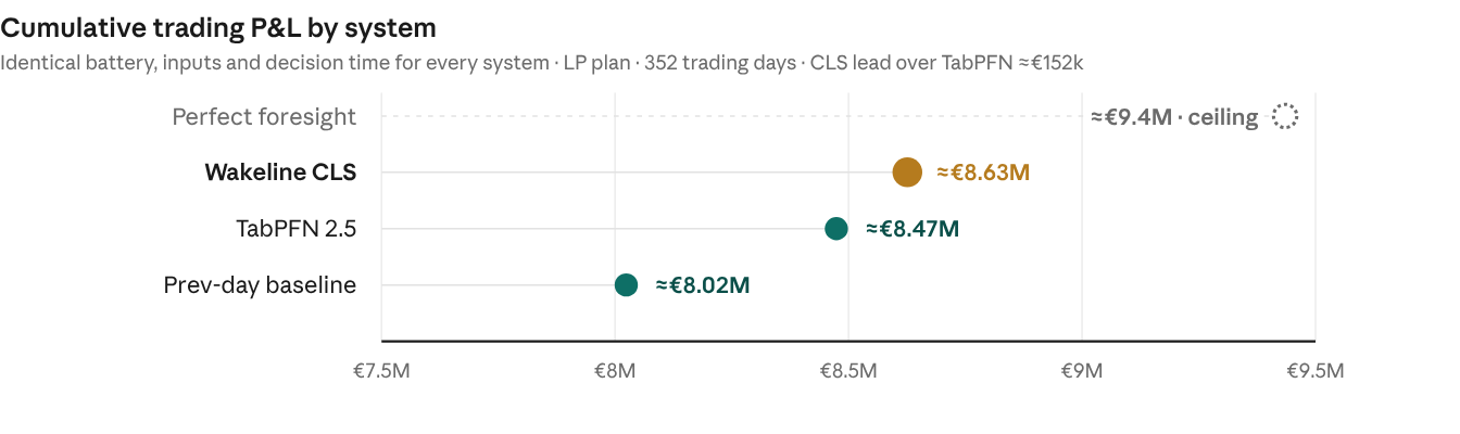
Key results at a glance
With the same inputs the CLS earns more than TabPFN under an optimising battery plan, trades the same volume, and has the higher forecast error, by the same ratio as in July. All systems receive the same external forecasts.
| System | Type | P&L ratio (CLS / benchmark)1 | Throughput ratio | Forecast MAE ratio3 |
|---|---|---|---|---|
| Perfect foresight2 | Theoretical ceiling using realised prices as the forecast | ~0.91xceiling | ~1.01xceiling | n/a |
| Wakeline CLS (reference) | Continually learning architecture; entered the backtest untrained | 1.00xreference | 1.00xreference | 1.00xreference |
| TabPFN 2.5 | Transformer-based foundation architecture for tabular prediction (Nature, 2025), given the same external forecasts | ~1.02xCLS ahead | ~0.99xparity | ~1.22xCLS behind |
| Previous-day persistence | Naive baseline: tomorrow equals today | ~1.08xCLS ahead | ~1.01xparity | ~0.75xCLS ahead |
1 Simulated battery revenue under the LP plan (primary), CLS divided by the benchmark: above 1.00 the CLS earned more. Against TabPFN the difference is +433 EUR per day, 95% interval +159 to +710; under the bidding rule the two are level (~1.01x).
2 Perfect foresight plans on the realised prices and marks the theoretical maximum; the CLS captured 91% of it under the LP plan.
3 Mean absolute error of the 96 quarter-hour prices, CLS divided by the benchmark: below 1.00 the CLS was more accurate pointwise, above 1.00 less accurate. The P&L and MAE columns read in opposite directions, so each cell carries a plain verdict.
| CLS, current, against | LP plan, EUR per day | Bidding rule, EUR per day | Spread captured, points |
|---|---|---|---|
| TabPFN 2.5 | +433 [+159, +710],better on 56% of days | +227 [−900, +1,383] | +2.0 [+0.8, +3.1] |
| Previous-day persistence | +1,711 [+1,361, +2,084] | +2,679 [+1,362, +4,000] | +10.6 |
On the simulated 200 MWh / 100 MW battery the LP plan’s perfect foresight is worth 26,804 EUR per day, the bidding rule’s 26,249. Intervals: paired daily differences, 20,000 bootstrap resamples of days, seed 0; they cover which days fell in the sample, not run-to-run variation.
What this benchmark measures, and what it does not
The benchmark measures one function of the CLS, next-day price forecasting, through what the forecast is worth to a battery.
- Every method’s forecast of the next day’s 96 quarter-hour prices feeds the identical battery simulation. Revenue differences stem from forecast quality alone.
- The CLS produces forecasts only. It has no influence over the battery’s schedule, its constraints or its execution.
- The results are internal and have not been independently verified.
Two ways to trade the forecast. We score every forecast twice, because how a battery uses a forecast decides what a better forecast is worth.
| Aspect | LP plan (primary) | Bidding rule (secondary) |
|---|---|---|
| How the day is traded | A linear program plans the day’s charge and discharge on the forecast, starting and ending empty; the planned volumes are executed at the realised prices | A fixed heuristic bids around the forecast; bids execute only where they clear against the realised price |
| What it uses | The whole curve: the relative price of every quarter-hour | Mainly the few cheapest and dearest quarter-hours and the price level |
| Where it comes from | The economics our forecasting pipeline has used in production since 24 September 2026 | The simulator of the July benchmark, kept for continuity |
The LP plan is primary because it is how the forecast is used in production; it was adopted before the analyses in this report. Both rules use the same battery: 200 MWh, 100 MW, 90% round-trip efficiency.
A new market to learn: 15-minute products
From delivery day 1 October 2025, the European Single Day-Ahead Coupling clears 96 quarter-hour prices per day instead of 24 hourly ones. For a forecasting system this is a new problem, not a finer version of the old one.
- Four times as many prices per day, each with its own position in the solar and load ramps.
- Quarter-hours within one hour now differ, most around sunrise, sunset and the evening peak, where the weather moves supply fastest.
- No 15-minute price history existed before October 2025. Every method in this benchmark starts its 15-minute history on the same day.
The July benchmark covered the hourly market from 2020 to September 2025, and its setup was built for 24 prices per day. For this report we rebuilt it for quarter-hours: the price and grid data at 15-minute resolution, a battery simulation that plans and settles 96 slots per day, and TabPFN as 96 per-slot models instead of 24. This report covers the first year after the change, and the CLS entered it untrained.
Setup
Every method runs on the same data, at the same decision time, through the same two battery rules.
| Setting | Value |
|---|---|
| Simulated battery | 200 MWh, 100 MW (25 MWh per quarter-hour), 90% round-trip efficiency, 1 EUR/MWh degradation, 0.20 EUR/MWh market fees, at most 1.5 cycles per day |
| Decision time | 10:00 local time on the day before delivery, two hours before gate closure, for every method |
| Information | Only data published before 10:00 |
| Inputs | Day-ahead prices; load, wind, solar and cross-border flows; the TSOs’ day-ahead load forecast for the delivery day (ENTSO-E Transparency); weather forecasts for five German cities issued two days before each hour (Open-Meteo) |
| CLS | One replay from an empty state, 1 October 2025 to 11 October 2026, in the production configuration, one fixed set of versions throughout |
| Period scored | The 352 delivery days from 14 October 2025 to 9 October 2026 on which every method forecast and the previous day’s prices were complete |
The first two weeks are a warm-up, as in July. Days are excluded only where a method had no forecast or data was missing, for all methods alike.
What the CLS was tested against
TabPFN 2.5 is the benchmark that matters: in July it beat every classical time-series method we tested. We ran it twice, with the July inputs and with the inputs the CLS reads.
TabPFN 2.5 is a transformer for tabular prediction from Prior Labs, published in Nature in January 2025, carrying extensive offline pre-training. We ran it as in July, scaled to the new market: 96 independent regressors, one per quarter-hour, retrained every day on a rolling 60-day window.
| TabPFN variant | Features | What it adds |
|---|---|---|
| July features | 50: calendar, the previous day’s price levels and statistics, the last six hours of prices, recent load, wind, solar and net imports, the latest load forecast | The July benchmark’s feature set, at the 10:00 decision time |
| Equal inputs | 88: the 50 above, plus the delivery day’s TSO load forecast (8 features) and the CLS’s weather forecasts for the delivery day (30 features) | The two inputs the CLS reads that the July set lacks, from the same files the CLS reads |
Nothing was tuned on TabPFN’s side: the added features are daily statistics and four fixed hours, chosen before its run.
Previous-day persistence assumes tomorrow’s prices equal today’s. Perfect foresight plans on the realised prices and marks the maximum value available; no real system can reach it.
Where the setup favours one side
- Same decision time. Both forecast at 10:00 from data published before then.
- Same inputs in the primary comparison, as in July. With the July features instead, TabPFN lacks two inputs the CLS reads; “Why the distance to TabPFN shrank” shows what they are worth.
- The CLS started untrained. It has no pre-training and learned online from 1 October 2025. TabPFN carries its offline pre-training on synthetic data.
- The CLS’s final stage was developed on part of this year, see the limitations.
Results
Under the LP plan the CLS earned more than TabPFN with equal inputs in 10 of 13 months. TabPFN was ahead in June, July and August, when solar sets the price of most quarter-hours and the delivery day’s weather matters most.
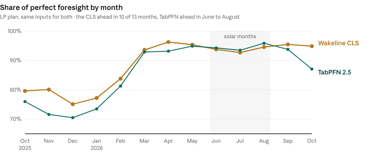
The lead was largest in the first four months after the switch to quarter-hours, 3.6 to 8.5 points of the maximum, while both methods were building their 15-minute history. Over the year the CLS was better on 56% of days. Under the bidding rule the same two forecasts are level: +227 EUR per day, interval −900 to +1,383.
Why the distance to TabPFN shrank
Both benchmarks compare like with like: in July neither system had external forecasts for the delivery day, here both have them. The distance shrank for two reasons: these forecasts are worth more to TabPFN than to the CLS, and the market had no regime shift comparable to 2022.
| What the delivery day’s external forecasts changed, 352 days | TabPFN 2.5 | CLS, final stage |
|---|---|---|
| How the system uses them | 38 extra features in each of its 96 per-quarter-hour models | In the final stage that turns the network’s curve into the published forecast |
| Forecast error | −23% | −12% |
| LP plan, EUR per day | +293 [+25, +559] | +304 [+221, +389] |
| Bidding rule, EUR per day | +1,608 [+274, +2,938] | +566 [−266, +1,398] |
- TabPFN turns the forecasts into error reduction more directly. Each of its 96 models, one per quarter-hour, already learns from the recent prices, grid data and calendar; the two forecasts enter as further inputs, and each model learns for its own quarter-hour how they move the price. On the 15-minute market, where solar ramps set the price of most daytime slots, that mapping is unusually valuable: TabPFN’s error fell by almost a quarter.
- The market changed. The July result was measured on hourly prices from 2020 to 2025, including the 2022 crisis, where the CLS’s advantage was largest. This year is a different market at a different resolution.
The July finding holds in its form: TabPFN has the lower error, by a ratio of 1.22 against 1.20 to 1.25 in July, and the CLS the higher revenue. The margin is smaller: the 14% lead of July has become a tie under the bidding rule (+1%, within noise) and a 1.8% lead under the LP plan, the rule that uses the whole curve.
The CLS improved during the year
Three versions of the CLS ran on identical data, decision time and simulator. Between them only the final stage changed, the step that turns the network’s learned curve into the published forecast; the network itself is identical in all three, bit for bit.
| Version | LP plan | Bidding rule | Error relative to version 1 |
|---|---|---|---|
| 1 | 90.3% | 79.7% | 1.00 |
| 2 | 90.2% | 82.1% | 0.96 |
| 3, current | 91.4% | 81.9% | 0.88 |
(Shares of the perfect-foresight maximum.)
- Version 2 improved the daily level: +624 EUR per day under the bidding rule, interval −38 to +1,344, and 4% less error. It is worth nothing to the LP plan.
- Version 3 brings the delivery day’s external forecasts into the final stage: +319 EUR per day under the LP plan, interval +234 to +408, better on 57% of days, and a further 8% less error. It is worth nothing under the bidding rule.
- Both changes are generic. They learn online from the realised prices like the rest of the CLS, with no rule specific to this market.
Why a higher error and a higher revenue coexist
TabPFN tracks the whole curve more closely; the CLS more often puts the day’s cheapest and dearest quarter-hours in the right place, and a battery earns its money from the spread between them.
| Measure, 352 days | CLS, current | TabPFN, equal inputs | Difference [95% interval] |
|---|---|---|---|
| Error of the daily level, ratio CLS / TabPFN | ~1.17x | 1.00x | CLS behind, interval excludes parity |
| Error of the shape around it, ratio CLS / TabPFN | ~1.14x | 1.00x | CLS behind, interval excludes parity |
| Correlation with the realised curve | 0.870 | 0.880 | −0.010 [−0.019, −0.001] |
| 4 cheapest + 4 dearest quarter-hours found | 45.5% | 42.0% | +3.5 points [+1.1, +5.9] |
| 8 cheapest + 8 dearest quarter-hours found | 61.2% | 58.9% | +2.2 points [+0.5, +3.9] |
| Share of the day’s possible spread captured, 8 + 8 | 89.3% | 87.3% | +2.0 points [+0.8, +3.1] |
A full charge or discharge of the simulated battery takes 8 quarter-hours. On exactly the slots it trades, the CLS is right more often, and that is worth more than the lower average error elsewhere on the curve. It is the explanation the July report gave, now measured on the extreme quarter-hours directly: pointwise accuracy is not the dominant determinant of economic value.
Known limitations
The CLS’s final stage was developed on part of this year. Its current design was fixed in October 2026 after tests on April to September 2026, so its gains partly reflect the data it was designed on. In October to March, months that design never used, the current version still earned +214 EUR per day over version 2 (interval +109 to +332) and +605 over TabPFN with equal inputs (+199 to +988). In April to October its lead over TabPFN is +277, interval −79 to +677. No part of this report is pre-registered.
The lead depends on how the battery trades. Under the LP plan the CLS leads TabPFN with equal inputs clearly; under the bidding rule the two are level. Both rules are reported throughout.
Higher error. TabPFN keeps the lower average error with equal inputs, error ratio about 1.2 as in July, in both the daily level and the shape. Applications where absolute accuracy matters directly should read the MAE ratio, not the revenue columns.
TabPFN was not tuned. Its added features are simple daily statistics of the CLS’s own inputs. A different encoding of the weather could make it stronger; we did not search for one.
One year, one market, one battery. 352 trading days on DE-LU, a 200 MWh / 100 MW battery. The intervals cover which days fell in the sample, not run-to-run variation. The CLS replay is deterministic on a given machine; TabPFN’s equal-input run gave the same error on two machines and two library versions (within 0.3%).
A backtest sees complete data. The replay runs on data as it was eventually published. A live system meets missing and late publications that a backtest does not, and these results say nothing about live performance.
Frequently asked questions
Why did you repeat the benchmark?
Our July benchmark was built for the hourly market. Since 1 October 2025 the European day-ahead market clears 96 quarter-hour prices per day instead of 24, so the data, the forecasts, the battery simulation and the TabPFN setup all had to be rebuilt. This report is the benchmark repeated from scratch on the first year of 15-minute trading.
Were these results independently verified?
No. They were produced internally by Wakeline GmbH. The setup is documented on this page, and we share the detailed benchmark reports in direct conversations so the methodology can be assessed in depth.
Is the trading strategy part of the CLS?
No. The CLS produces price forecasts only. The battery’s schedule comes from a fixed optimiser and, as a second check, from the bidding rule of the July benchmark; neither belongs to the CLS, and both treat every forecast identically.
Why is the CLS forecast error higher than TabPFN’s while its revenue is higher too?
A battery earns its money from the spread between the cheapest and the dearest quarter-hours it trades. TabPFN tracks the whole curve more closely; the CLS more often puts the extremes in the right place: it found the day’s 4 cheapest and 4 dearest quarter-hours 3.5 points more often. On the slots the battery trades, that outweighs the lower average error elsewhere.
Why is the lead over TabPFN smaller than in July?
Two things changed. The market: the July period included the 2022 energy crisis, the regime shift in which the CLS’s advantage was largest, as a system built to adapt when the market changes is designed to do, while the past year had no comparable shock apart from the switch to quarter-hours itself, and the CLS’s lead was largest right after that switch. The inputs: in July neither system had external forecasts for the delivery day; here both receive the grid operators’ load forecast and weather forecasts, and TabPFN gains more from them than the CLS, its error falling by almost a quarter. We cannot separate the two effects without rerunning the hourly period.
Why two battery rules, and which one counts?
How a battery uses a forecast decides what a better forecast is worth. The LP plan, which optimises the day’s schedule on the whole curve, is the primary measure because it is how forecasts are used in production. The July benchmark’s bidding rule is reported alongside for continuity.
Did TabPFN get the same information as the CLS?
Yes, in the primary comparison: the same price, grid and weather data from the same files, the same decision time of 10:00 on the day before delivery, and nothing published after it. The run with TabPFN’s July features is shown only as a reference.
Which market and period were tested?
The German-Luxembourg day-ahead market (SDAC), 352 trading days from 14 October 2025 to 9 October 2026, with a simulated 200 MWh / 100 MW battery.
Does the benchmark cover the whole CLS?
No. It evaluates one function, next-day price forecasting, through what the forecast is worth to a battery. The CLS’s other capabilities are covered in our research reports.
Can we see the full benchmark reports?
Yes, in direct conversations. They contain the complete simulator mechanics, the benchmark implementation details and the diagnostics behind every figure on this page.
Disclaimer
All results on this page were produced internally by Wakeline GmbH and have not been independently verified. Figures are approximate and rounded. The battery trading simulation exists to monetize forecast quality under realistic constraints; it does not represent a live trading system, and nothing on this page constitutes a forecast of live performance or an investment recommendation. TabPFN is published by Prior Labs. We report its results under the configuration documented in our benchmark reports, which we share in direct conversations.
Sources
- The CLS Forecasting Benchmark: Continual Learning Measured in Euros, Wakeline, 4 July 2026: the hourly benchmark this report follows.
- Market and grid data: ENTSO-E Transparency Platform (SDAC day-ahead prices, load, generation, cross-border flows, the TSOs’ day-ahead load forecast). Weather forecasts: Open-Meteo, forecasts issued two days before each hour, five German cities.
- TabPFN 2.5 by Prior Labs (v2.5 regressor weights, tabpfn 6.2.0 and 6.3.1).
Related articles
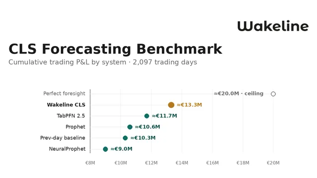
The CLS Forecasting Benchmark: Continual Learning Measured in Euros
The CLS forecasting function delivers approximately 14% higher cumulative trading P&L than TabPFN over 2,097 trading days on the German-Luxembourg day-ahead market. We present the benchmark results, methodology and limitations.

Measuring What Moves: Evaluation and the Problem of Time in Learning Systems
Static benchmarks measure a system at a single moment. Continual learning asks how performance holds as conditions drift, which is why evaluation has to account for time and consequence.
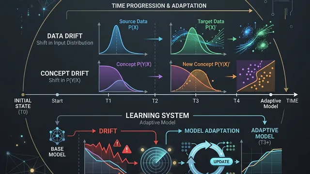
When Change Happens: Understanding Drift in Learning Systems
Learning systems face challenges when the statistical patterns of the world evolve faster than the model can adapt. We explore data, label, and concept drift.

Investment Opportunities
We are currently engaging with investors and strategic partners interested in long-term technological impact grounded in scientific discipline.
Wakeline represents a fundamentally different approach to artificial intelligence, prioritizing continuous adaptation, reduced compute dependence, and real industrial application.
Conversations focus on collaboration, evidence building, and shared ambition.