

Forecasting Traffic Without an Offline Training Phase
A continuous learning system matches the mean absolute error of the graph deep-learning models on the standard traffic benchmark without an offline training phase, by learning as it runs
Abstract
In Learning while the world changes we showed our Continuous Learning System (CLS) finding its way through a simulated town, learning from each delay it met. The traffic in that demonstration was synthetic, so the next question was the obvious one: what does the same system do on real roads, measured the way the field measures? We put its forecasting component, unchanged, on the PEMS-BAY and METR-LA benchmarks published with DCRNN. It has no offline training phase and no neural network; it learns from the stream as the stream arrives and goes on learning as long as data arrive. On its first registered run it landed in the range of the published graph deep-learning models on PEMS-BAY:
| PEMS-BAY test portion, MAE in mph | 15 min | 30 min | 60 min |
|---|---|---|---|
| CLS forecaster | 1.285 | 1.585 | 1.830 |
| Graph WaveNet, published | 1.30 | 1.63 | 1.95 |
| DCRNN, published | 1.38 | 1.74 | 2.07 |
| DCRNN, the authors' trained checkpoint, scored on the same samples | 1.309 | 1.644 | 1.958 |
- Below the published figures and the checkpoint at every horizon on mean absolute error, on 30 to 35 of 37 test days; on root mean square error behind both at 15 minutes and ahead at 30 and 60.
- On METR-LA, the harder network, within 3.6, 3.2 and 1.9 percent of the checkpoint. The graph models arrive on the test portion with the network's structure already extracted by training; the forecaster arrives with nothing and extracts it as it goes, and the gap narrowed week by week through the test portion, from 4.8 percent in the first week to 1.2 in the fourth at 15 minutes.
- The graph models are trained once and deployed as they are; ours keeps learning through the test weeks. A copy of ours frozen at the same point, a state it was never meant to be in, scores five percent behind the checkpoint, and the cost of staying frozen grows: 8 to 12 percent after five weeks, 16 to 29 percent after three months of the same network in 2022, and in Christmas week the frozen copy is worse than holding the current speed.
- Taken apart, the forecaster's learned part, which inputs matter and how to correct its own errors, is worth 3.5 to 14 percent over a plain nearest-neighbour look-up on the same inputs; the calendar carries most of the 60-minute forecast and the road neighbours add 3 percent on METR-LA.
- What this leaves: a small component that was never trained and was not built for traffic, running on a CPU, reaches the accuracy the field obtains from large graph networks designed for traffic and trained offline on GPUs, and it does so by staying in contact with the stream. Stop the contact and the forecaster's accuracy decays. The graph model never had it, and its accuracy decays the same way as the road moves away from what it learned. The structure these models extract in training does not have to be learned in advance and stored; it is available, continuously, from the road itself, to a system that keeps learning from it. On the Bay Area network that structure is, for the most part, each sensor's recurring daily pattern and its departures from it, which is what the forecaster learns; it does not reason about traffic, and the report claims nothing of the kind.
Every test was pre-registered and each test portion scored once per arm; the failed predictions are counted in the appendix. Results are internal and have not been independently replicated.
1. How we got here
The September demonstration ran on simulated traffic: a town of sixteen junctions, roadworks on a familiar route, a learner choosing its next turn and changing its choice as experience accumulated. It was built to make the learning visible, and the traffic in it repeated. It could not say how good the forecasts would be on real roads, or how the forecaster compares with the systems the field has measured for a decade. The standard way to ask that is the benchmark, so we registered a run on PEMS-BAY and METR-LA, the two datasets published with DCRNN, with the forecaster exactly as it was.
It landed in the graph models' range on PEMS-BAY at the first attempt and behind them on METR-LA. That raised the questions the rest of this report answers. The obvious objection first: our forecaster keeps learning through the test weeks and the graph models do not, so how much of the result is that? Then the fairness question it leads to: what if the graph model is given the same? That is not how the published models are used. In their papers and in the benchmark they are trained once and scored frozen; nothing in the protocol updates them, and no published variant of them learns from the test weeks. To ask the question at all we had to build a way for a graph model, deployed as its authors deploy it, to keep learning, and we did it with the cheapest means that respects the protocol's information cutoff: a correction layer on top of the checkpoint, learning only from outcomes already revealed. Then the question about the component itself: which of its parts carry the result, and would a plain look-up on the same inputs do as well? And underneath them, the belief our work rests on, argued in Why Weights Are the Wrong Place to Store Experience and Measuring What Moves: that a system in a changing environment improves on the dimension that matters only if it stays coupled to the consequences of its own predictions, and that this coupling, not a large model trained in advance, is where the useful structure lives. Each of the questions above is a way that belief could have failed. A benchmark administered once measures a sealed artifact at one moment; this report gives the standard number first, and then what happens to it in the weeks and months that follow.
2. What was tested
The component. The forecaster is a building block of CLS, our continuous learning system, and a general-purpose forecaster for any set of numeric streams; here each stream is one sensor's 5-minute speed. What it sees for a sensor at each step is the sensor's current speed, its means over the last 15, 30 and 60 minutes, its speed a day and a week earlier, the current speed and short means of up to four neighbouring sensors, and the time of day and week. From the outcomes that follow, it learns which of those inputs matter for that sensor and corrects its own systematic errors, online, at every step. Four is the component's cap on how many other streams it will take as influences, a fixed setting and not a traffic choice; the adapter hands it the nearest sensors by road distance, downstream and upstream alternately, and it keeps the first four. The graph models, by contrast, read every connected sensor through the road graph. On PEMS-BAY the time of day and week came to dominate what it attends to and the neighbours counted for little; on METR-LA the neighbours counted for three to four times as much. Its settings were fixed on development data before any test portion was scored, and not changed. Nothing in it refers to traffic. A full run over PEMS-BAY takes about eight minutes on a 16-core workstation without a GPU; the component is about a thousand lines of plain numerical code, and neither it nor its design is disclosed here. It learns at every step; "no training phase" means no conventional offline phase before deployment.
What "online" means. The forecaster sees each row once, in order, and uses only rows up to the current one; its test forecasts are made while it goes on learning from outcomes already observed. Cutting the data at any row leaves every earlier forecast unchanged bit for bit, checked on the held-out runs.
Benchmarks and protocol. PEMS-BAY, 325 sensors in the Bay Area, 1 January to 30 June 2017; METR-LA, 207 sensors on Los Angeles freeways, 1 March to 27 June 2012; both as published with DCRNN [1], under the standard protocol: chronological 70/10/20 split, MAE, RMSE and MAPE in mph at 15, 30 and 60 minutes ahead, zero readings excluded, the published metric code.
Comparators. Graph WaveNet [2] as published numbers; DCRNN as published numbers and as the authors' trained checkpoints (repository commit 602afd9), re-implemented for inference and run on our test samples; the checkpoints score better than the papers' tables and are the fair comparison. Three references run alongside: the current speed held (LAST), which cannot drift; a now-to-typical blend (BLEND), a running time-of-day profile mixed with the current deviation by one coefficient per horizon fitted on the training days; and our earlier forecaster (ENS), a per-sensor forecaster learning online.
Two arms. The live forecaster learns through the whole stream. The frozen forecaster learns from exactly the rows the DCRNN authors trained on, then stops learning of every kind. The two "frozen" states are not alike. For the graph models, trained once and deployed as trained is the normal state, the one their papers report and the one their complexity exists to hold up in; for our forecaster, which carries little knowledge of its own and reads the road as it goes, frozen is an intervention, a state it was never meant to be in. A comparison between the live forecaster and a graph model as deployed is a comparison between two adaptation protocols, and is labelled as such.
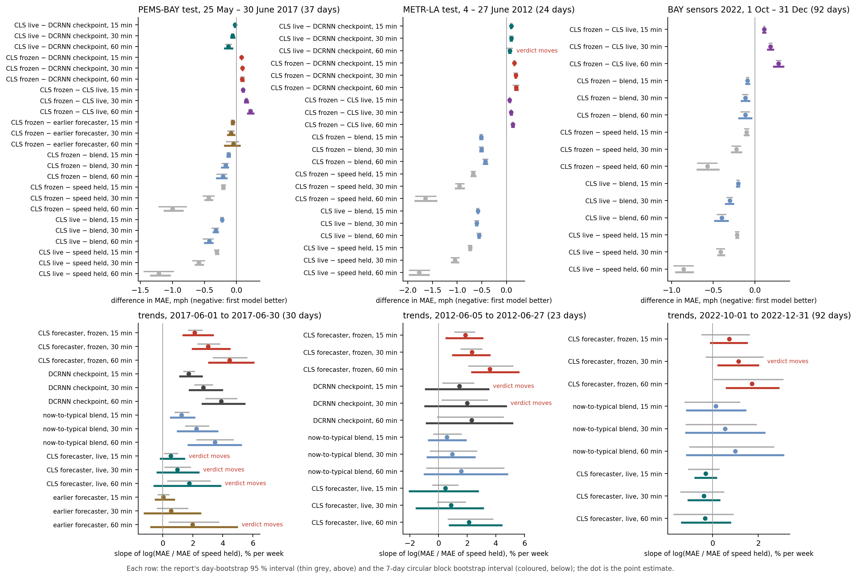
What is measured. Differences are paired by test day, 37 days on PEMS-BAY and 24 on METR-LA, with 95 percent bootstrap intervals over days, computed twice: with days resampled independently, as registered, and with a circular block bootstrap over 7-day blocks (3, 5 and 10 days as a sensitivity). The text quotes the day interval and says where the block interval changes the reading; Figure 3 shows both. Decay is measured as the slope per week of error relative to LAST, weekday effects removed, and as the gap between the frozen and live forecaster, which share every input and differ only in whether they learn; the second is the registered decay measure. Percentages of that gap are relative to the live error.
Pre-registration, and what was known when. Each study fixed configuration, code hashes, comparators, pass criteria and numerical predictions in a document sealed by its SHA-256 hash before the corresponding test portion was scored; predictions are graded on their literal wording in the appendix, and each run's record carries the time of its go. The forecaster's configuration was chosen on PEMS-BAY validation rows and on development data from a second domain, so PEMS-BAY test is a confirmation for it; METR-LA played no part in the design. The order of events, with every scoring of a test portion:
| date (2026) | what was scored | status of the hypothesis |
|---|---|---|
| 18 Oct | our earlier forecaster (ENS) on PEMS-BAY test | confirmatory for ENS |
| 18 Oct | an earlier hand-tuned forecaster on PEMS-BAY test | confirmatory for that component; its result is the forecaster's registered pass threshold |
| 18 Oct, 20:44 UTC | the forecaster on PEMS-BAY test and December 2022 | confirmatory; PEMS-BAY test scored for the third time in our work |
| 18 Oct | the forecaster on METR-LA test | confirmatory; METR-LA's first scoring |
| 18–19 Oct | two components of ours not described here, on PEMS-BAY test | confirmatory for them; fourth and fifth scoring |
| 19 Oct, 05:55 UTC | frozen and live arms on both test portions and the 2022 trace | hypotheses formed after the live results; predictions fixed from a pilot on training and validation rows (sixth and seventh scoring) |
| 19 Oct, 12:13 UTC | six ablation arms on METR-LA validation rows and an untouched 2022 window | no test row |
| 19 Oct, 13:28 UTC | corrected checkpoints and refreshed-forecaster arms on both test portions | the question came from a reviewer of a draft; predictions fixed from a pilot on development rows (eighth scoring) |
| 20 Oct | neighbours' forecasts, and raised neighbour caps, on METR-LA validation rows and the 2022 summer window | no test row; registered bars for a test run not met or not taken |
| 20 Oct | unusual-day events re-read from the saved predictions of every arm | no new model run, no new scoring; event definition and predictions registered before any error was read |
3. Results
3.1 First contact: PEMS-BAY
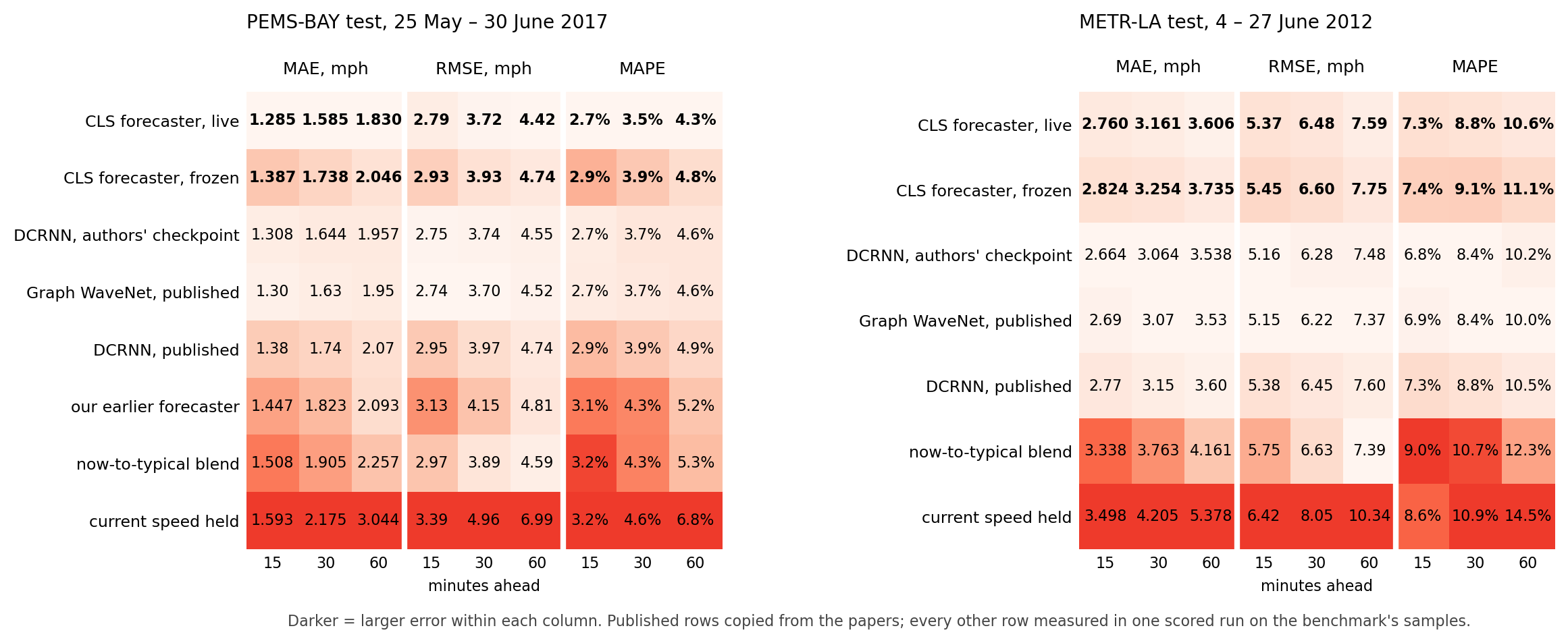
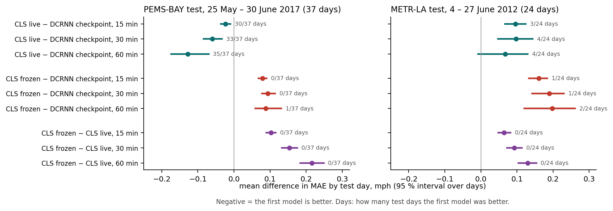
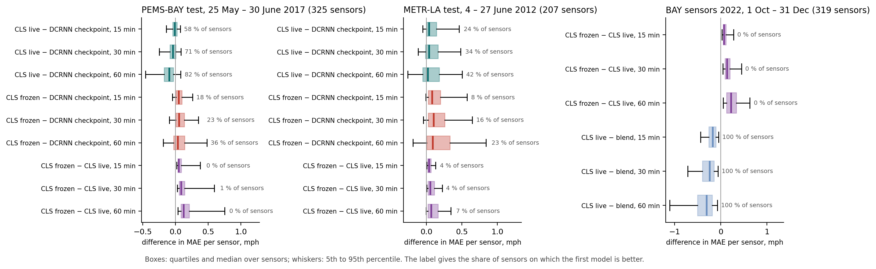
The live forecaster is ahead of the checkpoint at every horizon with the interval clear of zero, on 30 to 35 of 37 days; at 15 minutes the 7-day block interval ends at −0.002 mph, the thinnest result in this report, and the advantage lives in June and on free-flowing sensor-hours: in the Memorial Day week the checkpoint is ahead. The frozen forecaster is behind the checkpoint at every horizon, better on at most one day in 37, and behind its live twin on all 37 days; the frozen deficit is larger than the live advantage, so all of the live advantage comes from what the forecaster learned during the test weeks. Per sensor (Figure 4), the live advantage is a majority result that grows with the horizon, 58 percent of sensors at 15 minutes and 82 at 60; freezing costs on every sensor, with a long tail: the sensor at the 95th percentile loses 0.41, 0.62 and 0.77 mph.
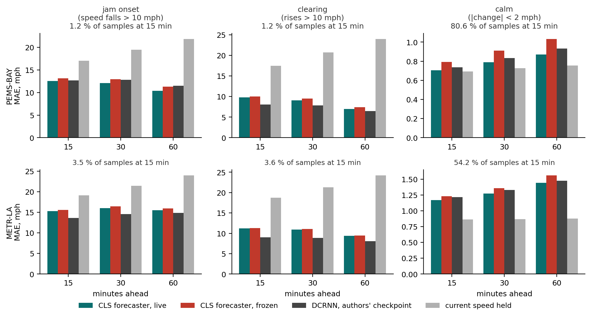
When a jam begins, the live forecaster and the checkpoint are equally bad, both about 12 mph too fast at 15 minutes. When a jam clears, the checkpoint is clearly better. On calm roads, where four samples in five are, the live forecaster is better than the checkpoint and close to the held speed, which that class favours by construction. Freezing costs most on calm roads, 13 to 18 percent, and least on onsets: a frozen forecaster gets the everyday level of traffic wrong, not the rare events. The worst day for both forecaster arms is Memorial Day, forecast as a weekday (60-minute MAE 1.74 live, 1.12 for the checkpoint, 1.26 for the held speed); the forecaster has no holiday calendar, and does not carry the bad day forward.
3.2 The harder network: METR-LA
METR-LA is the harder benchmark: noisier readings (a 5-minute change of 4.4 mph standard deviation against 1.75), 2.3 times as many onsets and clearings, 12 percent missing readings in the test portion, and 42 percent of PEMS-BAY's history before the test. The forecaster does not reach the graph models here (Figures 1 and 2, right). Live, it is behind the checkpoint by 0.096, 0.097 and 0.068 mph, better on 3 to 4 of 24 days. At 60 minutes the day-resampled interval includes zero and the 7-day block interval does not: the difference is +0.11 mph on the 18 weekdays and −0.12 on the six weekend days, and resampling days independently varies a weekend share the test window fixes. The forecaster is behind at every horizon, and the registered criterion fails as written. It beats the blend and the held speed by a wide margin, and the frozen forecaster, 6 percent behind the checkpoint, still does.
The gap shrank through the test weeks, from 4.8 percent in the first to 1.2 in the fourth at 15 minutes, while the frozen forecaster's stayed between 5 and 6. The two sides of that comparison are not starting from the same place: the checkpoint arrives on the test portion with the network's structure already extracted by its training, and the forecaster arrives with only what it has read from the stream so far and goes on reading. Four weeks do not show whether the gap closes. On METR-LA it attends to its neighbours three to four times as much as on PEMS-BAY. DCRNN reads every connected sensor's last hour through the road graph; the forecaster reads four neighbours' current state, and on a network where congestion recurs less regularly that is the information it lacks. This is our best reading of the diagnostics, not a tested explanation. The checkpoint keeps onsets and clearings at every horizon (Figure 5); the forecaster is slightly better on calm roads.
3.3 Taking it apart, one: stop the learning
The first thing to do with a result like Section 3.1 is to object to it. The online model has seen more data than the graph model as deployed. It has; the frozen arm measures what the extra data are worth, week by week.
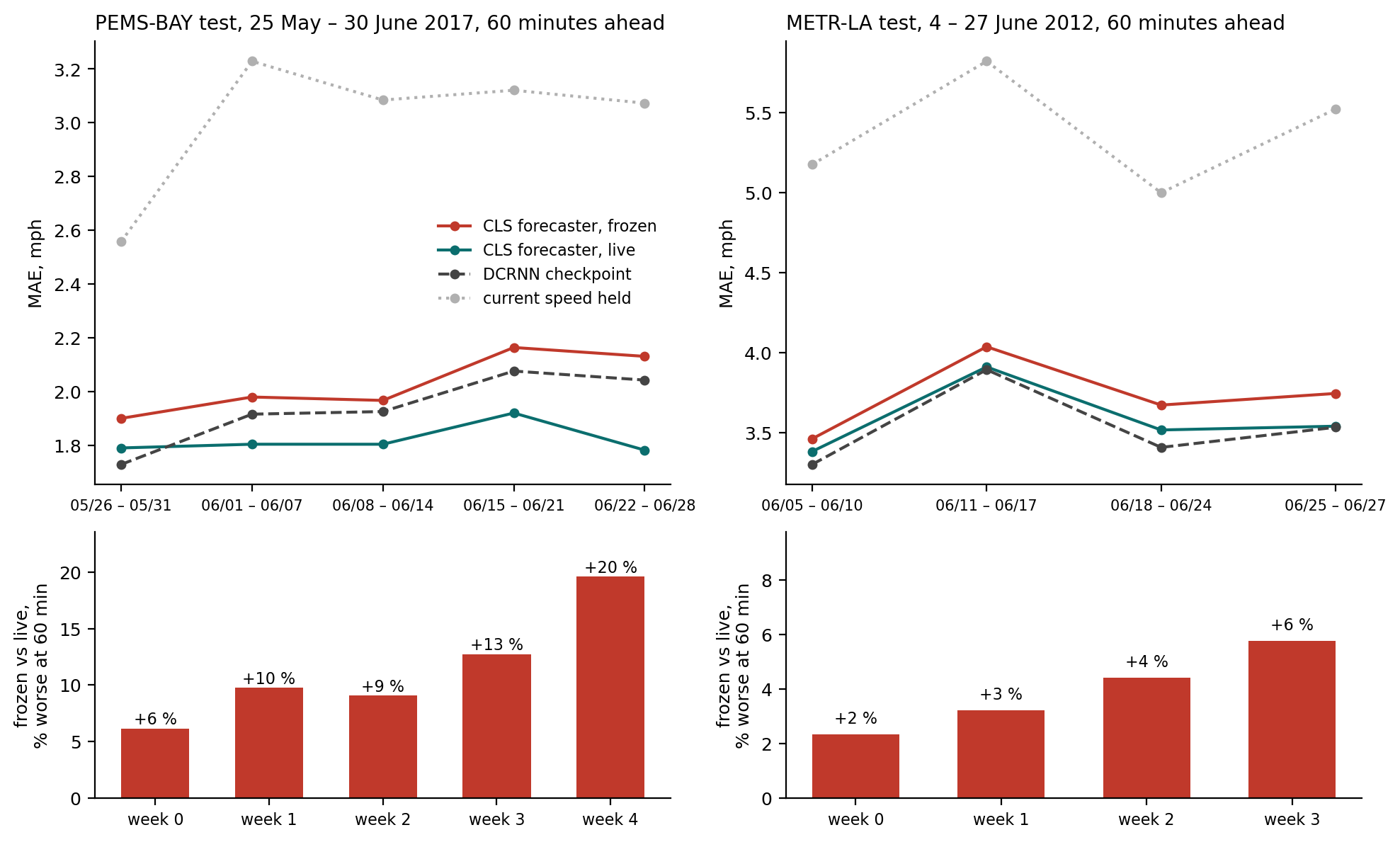
On PEMS-BAY the frozen forecaster is 6 percent worse than its live twin in the first test week and 20 percent worse in the last full one, 12 percent above its own first week while the live forecaster is level with its own. METR-LA shows the same shape over four weeks, from 2 to 6 percent.
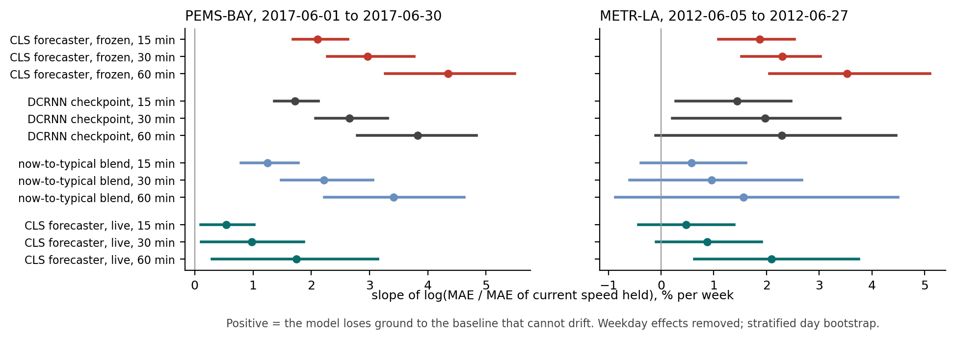
The frozen forecaster, the checkpoint and the blend lose ground to the held speed through June 2017 under both intervals; the live forecaster's slope includes zero under blocks. The end of the school year makes "nothing changes" a better guess, so a slope against the held speed is not drift alone. The clean measure is the gap between two copies of the same component that differ only in whether they learn: it grows by 0.022, 0.035 and 0.053 mph per week on PEMS-BAY and 0.038, 0.044 and 0.051 on METR-LA, every interval above zero. The frozen forecaster decays faster than the checkpoint, and that is the ordering the two designs imply. The graph model is built to be trained once and left alone, and much of its complexity exists so that it holds up when it is. Our forecaster is built to stay in contact with the stream and carries little general knowledge of its own, so a frozen copy of it is a forecaster in a state it was never designed for. Left alone, each decays as its design predicts: the checkpoint slowly, the frozen forecaster faster. The registration had taken its expectation from a pilot on development rows, where the frozen copy showed no trend, and had named the alternative in advance: that a slide against the held speed over June is a property of any model left alone on this network, not of the graph models. The alternative is what happened. On METR-LA only the frozen forecaster's decay is distinguishable from zero. Under this protocol, continuing to update the forecaster reduces its deterioration relative to a frozen copy by an amount that grows over the test weeks. The live copy takes in new observations, re-learns which inputs matter and corrects its own errors all at once; the experiment does not say which carries the benefit, nor how much of the frozen copy's loss is drift in the traffic rather than the plain value of more observations.
Five weeks is a short time to watch a model age, so we ran the same experiment on a public 2022 copy of PeMS District 4 data for 319 of the same sensors [3]: the forecaster learned from August to 30 September 2022, one copy was frozen there, and both forecast October to December.
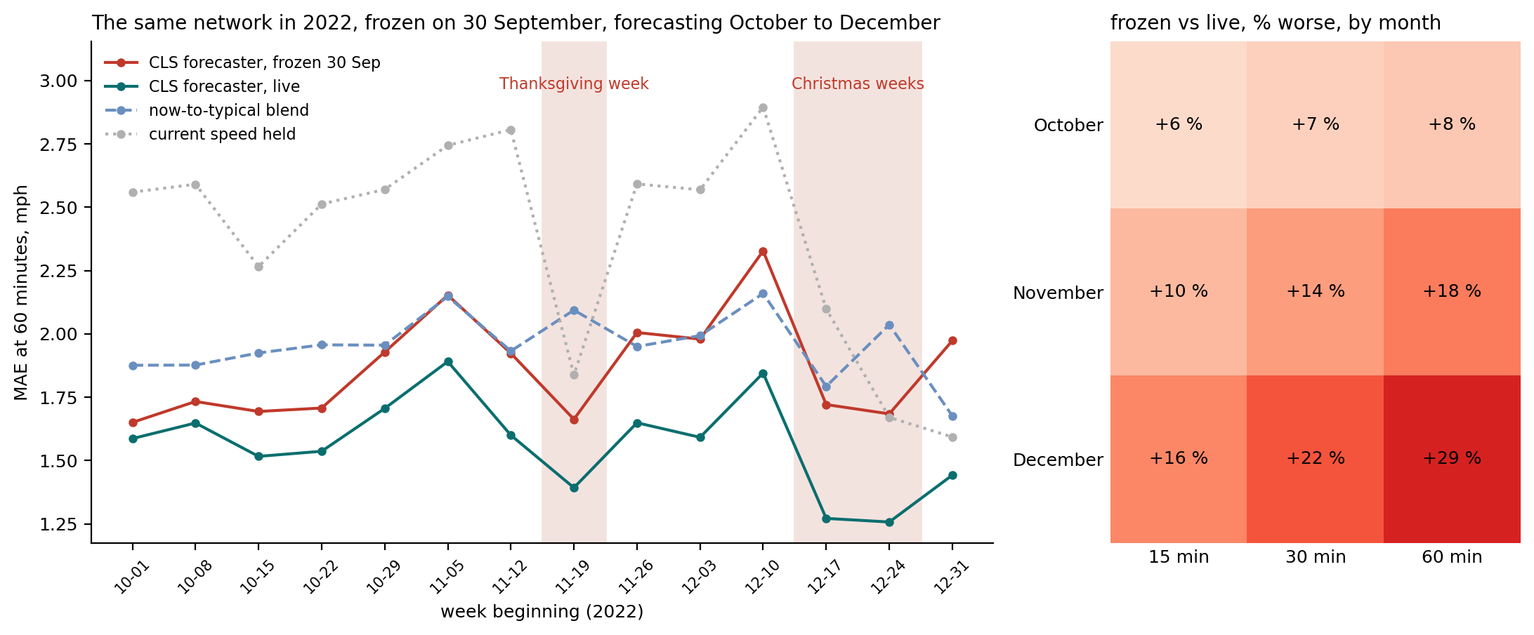
The cost of the snapshot rises every month at every horizon, from 6 to 8 percent in October to 16, 22 and 29 percent in December; over the quarter the frozen forecaster is worse on 91 of 92 days and still ahead of the blend and the held speed in every month. The loss is largest in the weeks that look least like the training weeks: Thanksgiving week, 12 to 19 percent, and the two Christmas weeks, 19 to 35. In the week of 24 to 30 December the frozen forecaster is worse than holding the current speed at every horizon; the live forecaster is 14 to 25 percent better than holding it. The frozen forecaster holds no situation from a week like that; by Christmas the live forecaster had stored Thanksgiving week.
Where, within a window, does the cost of losing contact sit? We had expected roadworks and closures: a road that changes and stays changed for days, which a forecaster in contact with the stream should learn within a day. The benchmarks carry no incident labels, so events were defined from the speeds alone and registered before any error was read: a sensor-day more than 10 mph below that sensor's own typical pattern for a quarter of the day, and an event two or more such days in a row with a normal day before them. Hard closures would appear as missing readings, and none did on the Bay Area windows.
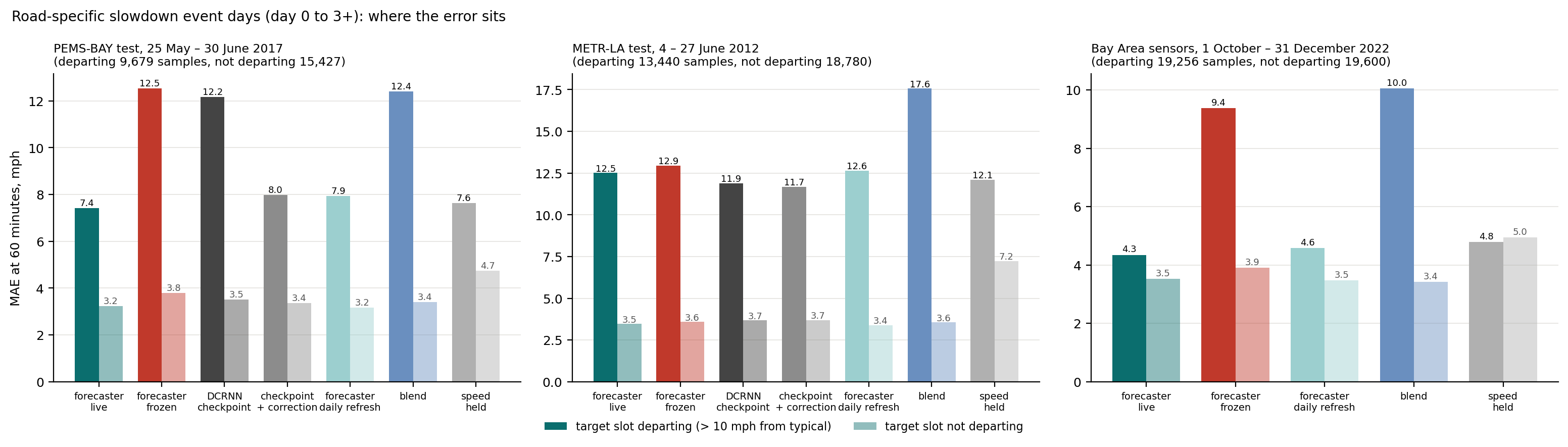
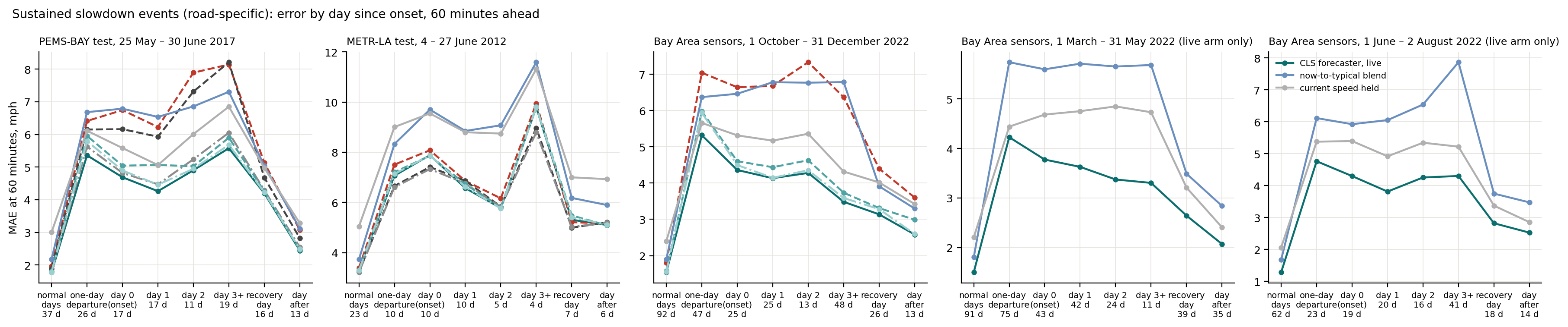
The expected picture did not appear; what appeared is simpler. On the Bay Area network, on the sensor-days of such events, the cost of being out of contact is four times its everyday size: the frozen forecaster is 49 and 74 percent behind the live one at 60 minutes in 2017 and 2022, against 12 and 18 overall, and the checkpoint as deployed 45 percent. But the gap is already there in the first hours of the first day, it is there on single bad days that persist nowhere, and it does not grow from the first day to the second; nor does the live forecaster lag when the road recovers. This is not a forecaster learning a changed road within a day. It is a forecaster in contact with recent outcomes handling any unusual day far better than one that lost contact. Figure 9 shows the mechanism: on the slots that depart from the typical pattern, the frozen forecaster, the checkpoint as deployed and the blend all forecast the typical pattern and are equally wrong, 12.2 to 12.5 mph; the live forecaster, its daily refresh, the corrected checkpoint and the held speed sit together at 7.4 to 8.0. The corrected checkpoint recovers most of that gap and not all of it: on continuation days it is 6.9 percent behind the live forecaster, interval [2.6, 11.3], where overall the two tie. Holding the current speed is strong on those days and beats the frozen forecaster. On METR-LA none of this appears. The events sit on about a dozen sensors per window, what the definition cannot tell apart (roadworks from a faulty detector or a seasonal change) heads the study's report, and eleven of its sixteen registered predictions failed, including the one the brief hoped for.
3.4 Taking it apart, two: give the graph model the same
If the gain is the updating, the graph model should get it too. Nothing in the published work does this: DCRNN and Graph WaveNet are trained once on the training portion and scored frozen, and the benchmark has no provision for a model that learns during the test weeks. So the arms in this section are ours, built so that the question could be asked. A graph model deployed as trained is the benchmark's protocol, not an operator's practice either; an operator can retrain on a schedule or put a lightweight correction on top of a deployed model. This section gives the graph model the second of those, and gives the forecaster an operator's refresh schedule, so that the comparison is between models kept current by different means. Retraining DCRNN itself on a schedule was out of scope. Two correction layers sit on the checkpoint's forecasts and learn only from revealed outcomes: an online error-correction rule taken from CLS, per sensor, indexed by level, time of day and recent change, and a per-sensor recursive-least-squares calibration. Two refresh schedules reopen the frozen forecaster once a week or once a day, let it learn from the interval's observations, and freeze it again. All of it was registered before any test row was scored.
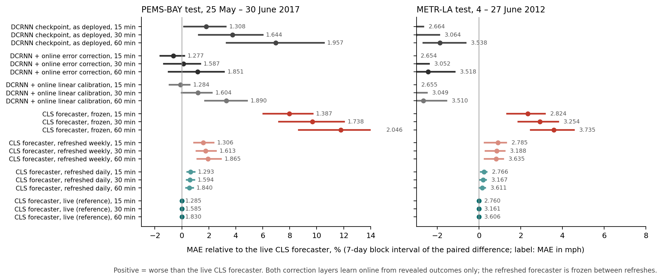
On PEMS-BAY the error correction takes 2.4, 3.5 and 5.4 percent off the checkpoint, the calibration 1.9, 2.5 and 3.4, every interval clear of zero. The corrected checkpoint and the live forecaster are then level, 1.277, 1.587 and 1.851 against 1.285, 1.585 and 1.830 mph, with intervals that include zero at every horizon; on RMSE the corrected checkpoint is ahead. We had registered that the forecaster would still beat it at 30 and 60 minutes; it does not, and the alternative the registration named, a tie everywhere, is what happened. Refreshing the forecaster once a day instead of continuously costs 0.6 percent; once a week, 1.6 to 1.9. A forecaster refreshed daily beats the checkpoint at every horizon; one refreshed weekly ties it at 15 and 30 and beats it at 60, and is behind the corrected checkpoint at every horizon. On METR-LA the corrections gain the checkpoint 0.3 to 0.8 percent and, since the forecaster was already behind, the corrected checkpoint is ahead of the live forecaster by 4.0, 3.7 and 2.7 percent, as registered. On the 2022 trace a weekly refresh costs 2.4 to 2.9 percent over the quarter and a daily one 1.2 to 1.5; the weekly arm's gap to live does not grow from October to December, and in Christmas week it is 2 to 3 percent behind live and ahead of the held speed, where the frozen copy was 19 to 34 percent behind.
The correction layers cost 1 to 5 seconds of computation for a test portion against 16 to 21 minutes for a forecaster arm; what they need is the trained checkpoint, and what the forecaster needs is the stream. On PEMS-BAY, staying current is worth about five percent whichever model does it, and the forecaster obtains it without an offline training phase. On METR-LA the graph model's advantage survives every way of keeping either model current that we tried.
3.5 Taking it apart, three: which parts of the forecaster carry it
The last question is about the component itself. Six arms of the forecaster ran live with parts removed through its public interface: the full forecaster; without the calendar; without the four neighbours; without its online error correction; with every input treated alike instead of learning which matter; and a plain nearest-neighbour look-up on the same inputs, the baseline a careful practitioner would build. They ran on rows the configuration was never chosen on and that are not the benchmark's test portion: the METR-LA validation rows (13 days, on which the DCRNN authors chose their checkpoint) and an untouched window of the 319 Bay Area sensors, 1 March to 31 May 2022 (92 days). Eleven of sixteen registered predictions failed in whole or in part, almost all because we over-predicted the cost of removing each part.
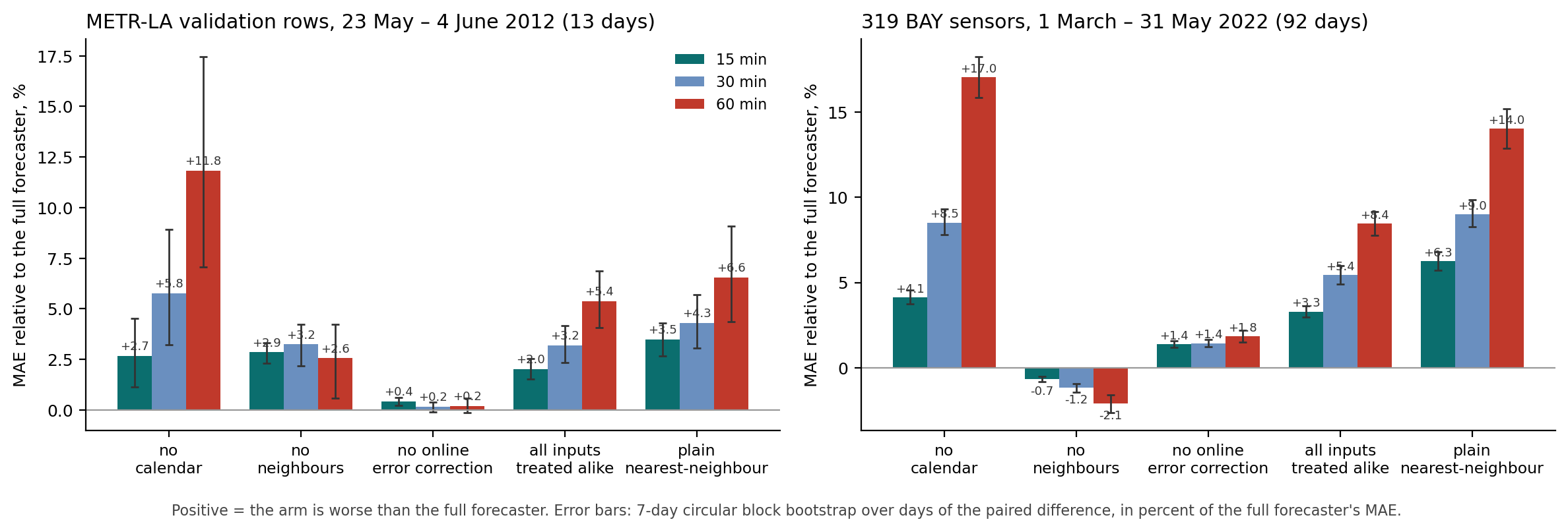
The plain look-up is 3.5, 4.3 and 6.6 percent worse than the full forecaster on METR-LA and 6.3, 9.0 and 14.0 on the 2022 window, a little over half of it from learning which inputs matter and the rest from the error correction and the read-out. The calendar is the largest single input at 60 minutes, worth 12 and 17 percent, and a small one at 15, worth 3 and 4; without a clock the forecaster turns to its neighbours, which carry the network's time signature, and on Memorial Day 2022 the clock-less copy is the better one. The neighbours have different signs on the two networks: worth 2.9, 3.2 and 2.6 percent on METR-LA, and on the Bay Area network removing them makes the forecaster better by 0.7 to 2.1 percent. The error correction is worth 1.4 to 1.8 percent on the Bay Area network and nothing on METR-LA. The description "an adaptive library of time-of-week patterns per sensor, corrected with recent observations" fits the 60-minute result and overstates the clock at 15 minutes.
One other way of giving the forecaster the road graph was tried under its own registration, on the METR-LA validation rows and on the untouched June–July 2022 Bay Area window, and on no test row: the forecaster's own forecasts for its four neighbours, fed back to it as inputs. On METR-LA the forecaster gains 1.0, 1.6 and 1.7 percent from them, on 12 to 13 of 13 days; four random sensors' forecasts gain it 0.5, 0.8 and 1.5, so part of the gain is a network-wide signal. The neighbour-specific difference is about half the gain at 15 and 30 minutes and an eighth at 60; on thirteen days its registered day interval includes zero at every horizon, the 5- and 7-day block intervals lie below zero at 15 and 30, and the forecaster attends to the neighbours' forecasts 2.6 times as much as to the random ones. The direction contrast held more clearly than predicted: two downstream neighbours' forecasts help more than two upstream ones, by a margin that grows with the horizon and is clear of zero at 30 and 60 minutes, and the 60-minute onset error falls 3.7 percent, almost all from the downstream arm. The road graph carries information the forecaster can use at 15 to 30 minutes, and it is directional, congestion arriving from downstream, the first such signal in any of our studies of neighbours. The registered condition for scoring the test portion was the day interval on the neighbour-specific difference, and it was not met, so this stays a validation result outside the claims of this report; with the forecasts the forecaster is still 5 to 6 percent behind the checkpoint. On the Bay Area network the same inputs neither help nor hurt, and the difference from random sensors' forecasts is three thousandths of a mile per hour or less.
3.6 Reading the forecaster
Everything the forecaster has learned can be read out of it, sensor by sensor, in the units it works in. That is a property the graph models do not have, and it is the same property our earlier reports relied on when they read a learned cost rule directly from the system rather than inferring it from behaviour. Two readouts are given here; both were read from the saved runs by an instrumented replay that reproduces every forecast bit for bit, and nothing was re-scored.
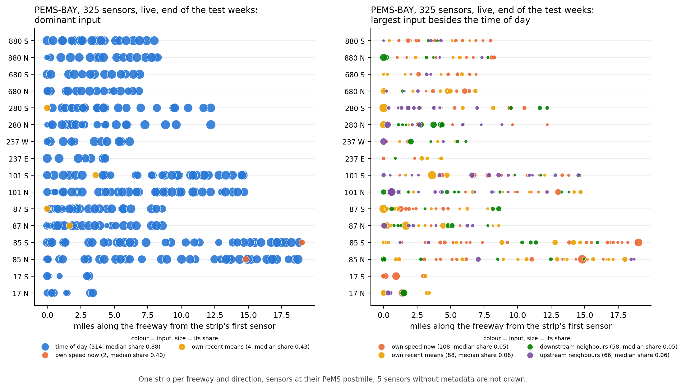
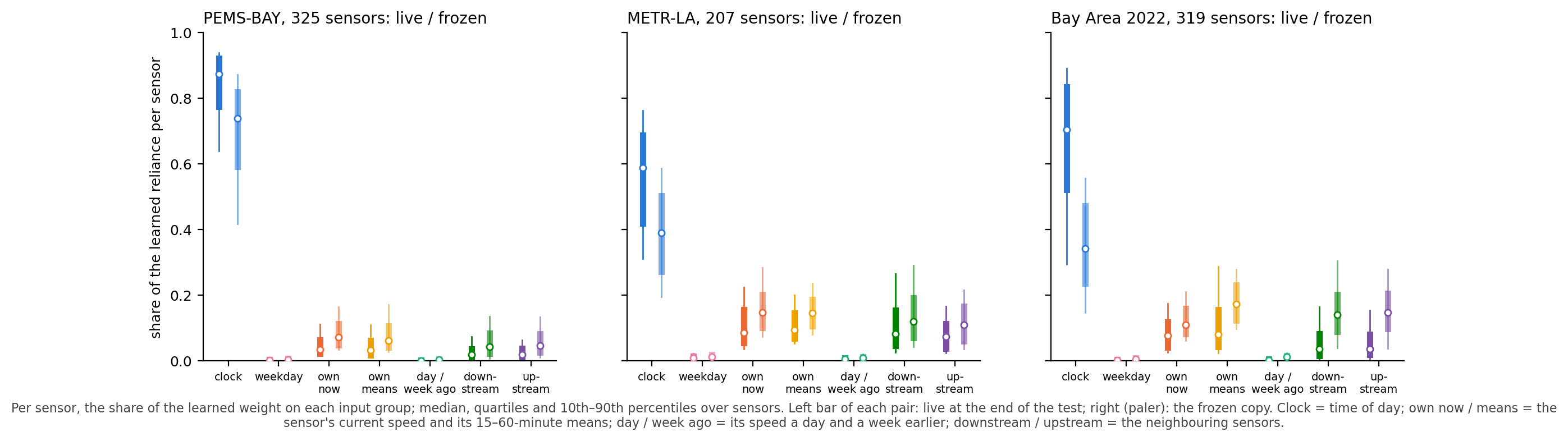
What each sensor's forecast relies on. For every sensor the forecaster learns how much each input matters; the result is a share per input that can be drawn on the road. The time of day is the largest input on 319 of 325 PEMS-BAY sensors and 189 of 207 METR-LA sensors, with a median share of 87 percent on PEMS-BAY and 59 on METR-LA; the day of the week is almost unused on both, weekends being told apart by their speed pattern. What is left is split between the sensor's own recent state and its neighbours, and the two networks differ in kind: on PEMS-BAY the median neighbour share is 4.5 percent, on METR-LA 17, where fifty sensors give the neighbours more than a quarter and the five that lean on them most all lean downstream. A few sensors run on their own state and not on the clock, 79 percent on one SR-85 sensor; the forecaster found them by itself. The reliance is not static: the clock's share rises through the whole run on all three data sets and had not levelled off when any run ended, from 73 percent at the freeze to 87 at the end of June on PEMS-BAY, and the frozen copy's reliance is an earlier point on the same curve. Part of the frozen copy's deficit in Section 3.3 is a less settled reliance, not only a shorter record.
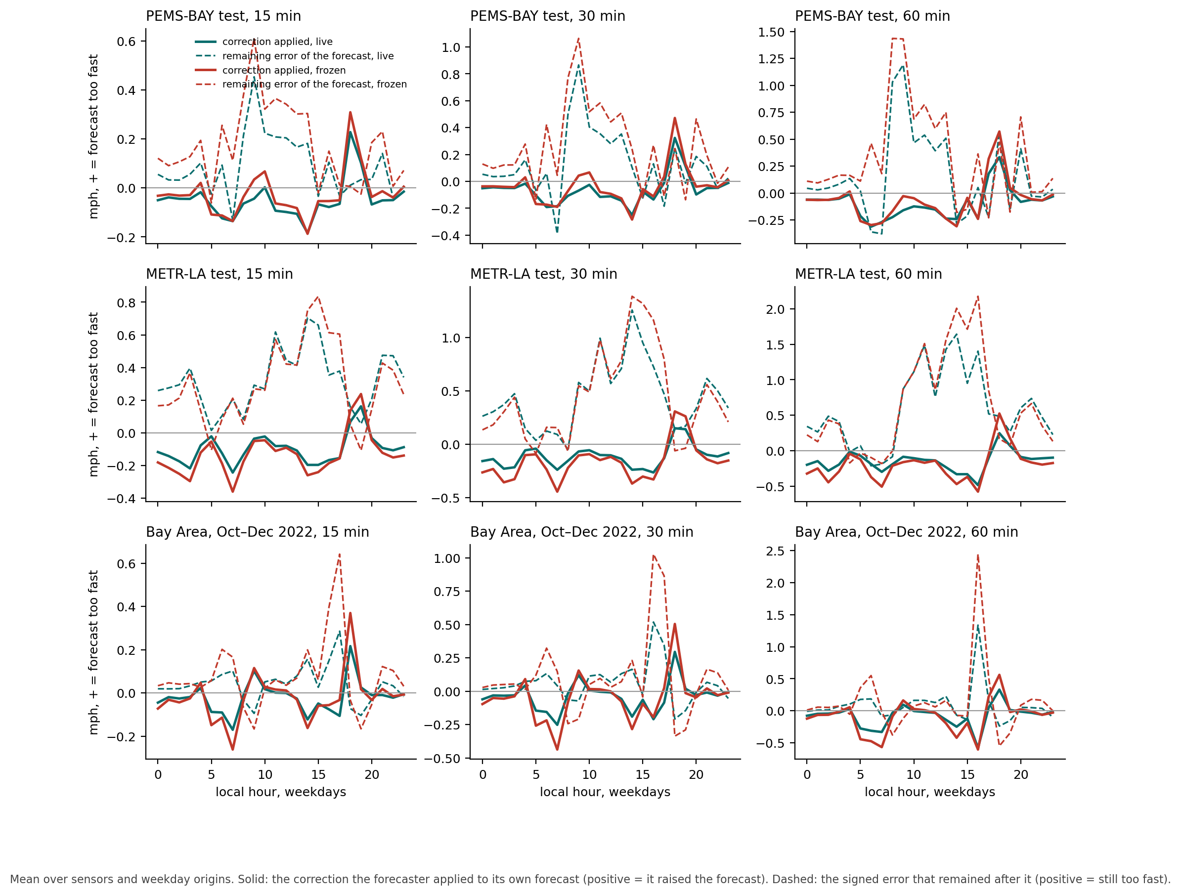
Where it knows it is wrong. The forecaster keeps, per sensor and horizon, a running account of its own systematic error by situation, and adds the correction to its forecast. Read at the situations that occurred in the test weeks, the account is small and points the right way: 0.3 to 1.2 mph held, about half of it applied, the sign almost always "run slower", largest in the morning and afternoon peaks. Where the remaining error is largest, at 9 o'clock on PEMS-BAY, the correction held was only 0.1 to 0.3 mph: the forecaster holds a correction in the right direction at the hours it is most wrong and applies too little of it. At jam onsets the forecast is 12 to 15 mph too fast and the correction applied was 0.4, forty times too small, because an onset is not a systematic error of the situation it is filed under. On METR-LA the forecaster applies no correction on half its origins and its account is twice as large; the sensor it corrects least holds corrections of 2.5 mph at midnight and applies none of them, which is right, since its measured error there is 0.4. Read as sentences, the account says things like: on sensor 400418, SR-87 north at Curtner Avenue, at six in the morning at 62 to 66 mph, the hour before its usual jam, subtract 3.4 mph. It knows the jam's edge is coming; it does not know when.
4. Limitations
Two adaptation protocols, not two architectures. The live forecaster learns from test-week outcomes already observed; the graph models were trained on seventy percent of the data and frozen. The frozen arm separates the effects, but its state came from one online pass and the checkpoint's from offline training with a checkpoint chosen on the validation rows. The correction layers of Section 3.4 were designed by us and tuned on nothing; a retrained DCRNN, or a better-engineered correction, was not run and could move the tie.
Design choices and exposure. The configuration was chosen on PEMS-BAY validation rows and another domain's development data; PEMS-BAY test has been scored eight times in our work, by this component and by others, each under its own registration. METR-LA played no part in the design. The frozen and adaptive arms were designed after the live results, from pilots on development rows. Graph WaveNet is present as published numbers only.
Statistics. Days are not independent, so every interval was recomputed with a 7-day block bootstrap (Figure 3). Eight of 105 verdicts change: the live forecaster's June slope, our earlier forecaster's at 60 minutes and the checkpoint's on METR-LA lose their support; the forecaster's 60-minute deficit on METR-LA and the frozen forecaster's 30-minute 2022 slope gain it. The independent evidence behind the live-versus-frozen comparison is closer to the number of weeks and regimes than to the number of forecasts; per-sensor distributions are descriptive.
One network, one season. PEMS-BAY's test weeks are late May and June 2017, METR-LA's June 2012, the 2022 trace one autumn; the ablations and the neighbour-forecast study ran on development-adjacent rows with thirteen METR-LA days. The neighbours' sign differs between the two networks, and one network cannot say whether that is the wiring, the season or the forecaster's use of four neighbours. A raised cap on neighbours, 8 to 16 instead of 4, was tried under its own registration on the same two windows: it gains 1.0 to 1.6 percent on METR-LA validation, most of the 60-minute gain being Memorial Day, and costs 0.3 to 1.1 percent on the Bay Area network, growing with the cap; it was not carried to the test portion. The road graph, read in some other way, is still the first place to look on METR-LA.
What "generic" means here. The learning mechanism is generic: nothing in it knows the data are traffic. The input handling is generic in that the same code takes any set of numeric streams, with its inputs built by one rule; the choice of neighbours by road distance is domain-informed. Generic forecasting capability across domains is not established here; the same configuration runs on a second kind of data, and that result belongs in its own report.
What it does not do. The forecaster does not anticipate the start of a jam, clears jams later than the checkpoint, and treats holidays as weekdays; none of this changed between the live and frozen arms or between the benchmarks.
Replication. All results are internal, hash-pinned and not independently replicated. The component is not released.
5. Conclusions
We moved a forecaster from a synthetic demonstration to the field's benchmark without changing it, and it landed in the graph models' range on the first registered run. Taking that result apart is what this report is about, and what the taking-apart leaves is this. A component of about a thousand lines, with no training phase, no neural network and nothing in it built for traffic, learning once through the stream on a CPU, reached the mean absolute error of graph deep-learning models designed for traffic, on PEMS-BAY. The structure they extract offline was available online, from the stream alone. A copy of it that stopped learning fell five percent short at once and twenty to thirty percent short within weeks and months, worst in the weeks the training data did not contain: the structure was not stored once and kept, it was re-derived from the stream as the road changed. And a graph model given the same coupling, a correction layer learning from revealed outcomes, drew level with the live forecaster: the coupling was what mattered, and the forecaster's contribution is that it supplies the coupling without a large trained model to correct. The model does not have to be big, and it does not have to be trained in advance. It has to stay in contact with the environment, and when it does, a small one is enough on this benchmark.
METR-LA marks where that stops being true. On a network with more non-recurrent congestion the graph model's wider view of the road is worth three to four percent that staying current does not recover. Giving the forecaster a wider view of its own, four times as many neighbours, recovers a fifth to a quarter of that gap on METR-LA validation rows, most of it on one holiday, and costs about one percent on the Bay Area network, where the neighbours carry nothing the clock does not; a wider view is not a setting one network would choose for the other. The first registered sign that the forecaster could read the road's direction came from giving it its neighbours' forecasts, on validation rows, outside this report's claims. What is not established is any advantage on a harder network, on the minutes when traffic changes fastest, over a graph model that is itself kept current, or beyond the two networks and three seasons tested here. The September demonstration showed the learning happening; this report measures it against the field, and finds that most of the result comes from continuing to learn.
All results were produced internally by Wakeline GmbH and have not been independently verified. Figures are approximate and rounded. This report describes a research system evaluated on public historical traffic data. It does not describe a deployed product, and no claim is made about the performance of any live system.
Appendix. Pre-registered predictions, graded
Verdicts are on the literal wording of each registration. The forecaster's held-out study (T), the METR-LA transfer test (F, X), the frozen control and decay study (P) and the adaptive baselines (A) are graded below; the sixteen ablation predictions (B) are summarised after.
| # | Expectation as written | Verdict |
|---|---|---|
| T1 | PEMS-BAY test at or below 1.02 × an earlier hand-tuned forecaster (1.357 / 1.711 / 2.006); predicted 1.33 / 1.66 / 1.93 ± 0.03 | Confirmed, 1.285 / 1.585 / 1.830; the prediction was pessimistic |
| T2 | December 2022: 15–30 % below LAST and 5–15 % below BLEND | Confirmed on the rule; the BLEND margin, 16–23 %, exceeded the range |
| F4 | METR-LA: at or below the trained DCRNN; expected to fail | Failed at every horizon, as expected; the 60-minute day interval includes zero, the block interval does not |
| F5 | METR-LA: at or below Graph WaveNet's published numbers; expected to fail | Failed, as expected |
| F6 | METR-LA: at or below DCRNN's published numbers; expected to fail | Passed at 15 minutes (2.760 against 2.77), failed at 30 and 60 |
| X1 | METR-LA MAE in 2.76–2.90 / 3.20–3.36 / 3.70–3.92 | Below the range at every horizon |
| X2 | METR-LA gap to the checkpoint +4 to +10 %, intervals excluding zero | Failed: +3.6 / +3.2 / +1.9 %; the 60-minute day interval includes zero |
| X5 | The neighbours' share of what the forecaster attends to on METR-LA ≥ 0.15 (PEMS-BAY 0.05) | Confirmed, 0.174 |
| P1 | Frozen PEMS-BAY MAE in 1.37–1.45 / 1.72–1.82 / 2.04–2.18 | Confirmed |
| P2 | Frozen forecaster worse than the checkpoint at every horizon | Confirmed |
| P3 | Frozen worse than Graph WaveNet everywhere and than DCRNN published at 15 min | Confirmed; at 30 and 60 min, open, it beat DCRNN's published numbers |
| P4 | Frozen beats ENS at 15 and 30 min | Confirmed; 60 min undecided |
| P5 | Frozen beats BLEND and LAST everywhere | Confirmed |
| P6 | Frozen / live − 1 in +7–13 / +9–15 / +12–19 %, worse on ≥ 33 of 37 days | Failed at 60 min by 0.2 points: +8.0 / +9.7 / +11.8 %, worse on 37 of 37 |
| P7 | No Memorial-week reversal | Confirmed |
| P8 | Frozen vs LAST over June: no trend at 15 and 30 minutes, and a June slope smaller than the checkpoint's at every horizon. The expectation came from a pilot on development rows; the registration added that if the frozen forecaster instead slides as fast as the checkpoint, the June slide is a property of models left alone on this network, not of the graph models | Failed on both clauses: +2.1 / +3.0 / +4.5 percent per week, faster than the checkpoint. The registration's alternative reading is the one the result supports |
| P9 | Live vs LAST over June: no trend at 15 and 30 min | Failed on the day interval (+0.5 / +1.0 %, intervals just above zero); undecided under 7-day blocks |
| P10 | The gap frozen − live grows at 60 min | Confirmed at every horizon |
| P11 | Last full week: frozen / live − 1 in +9–15 / +11–18 / +14–24 % | Confirmed, +11.9 / +15.4 / +19.6 % |
| P12 | METR-LA: frozen = live × 1.02–1.05 / 1.03–1.07 / 1.04–1.09; worse than every graph number | Comparisons held; the ratio missed at 30 and 60 min, the cost being smaller |
| P13 | METR-LA: frozen ≥ 10 % below LAST, below BLEND at 15 and 30 min | Confirmed |
| P14 | The frozen forecaster's gap to the checkpoint does not shrink over the METR-LA weeks | Confirmed, 1.009; the live forecaster's 0.971 |
| P15 | METR-LA: frozen vs LAST no trend; the gap grows at 15 and 30 min | Failed on the first clause (+1.9 / +2.3 / +3.6 %); the gap grew everywhere |
| P16 | 2022 frozen / live − 1 at 60 min: Oct +5–12, Nov +8–18, Dec +10–25 %, rising | December above the range, +28.5 %; the rise held |
| P17 | 2022: frozen beats LAST every month and BLEND in December | Confirmed |
| P18 | 2022: live December reproduces T2 bit for bit; frozen vs LAST positive trend at 60 min | Confirmed; at 30 min marginal (day interval includes zero, block interval does not) |
| A1 | PEMS-BAY: both corrections beat the checkpoint as deployed, by 1–5 / 1.5–5 / 2–7 % | Confirmed, 2.4 / 3.5 / 5.4 and 1.9 / 2.5 / 3.4 |
| A2 | PEMS-BAY: live forecaster beats the best corrected checkpoint at 60 min by 1.5–5 % and at 30 by 0.5–3 | Failed: +0.6 / −0.1 / −1.2 %, no verdict anywhere; the registered alternative, a tie, is what happened |
| A3 | PEMS-BAY: the two corrections within 1 % of each other | Failed: the error-correction rule is 0.5 / 1.1 / 2.1 % better |
| A4 | PEMS-BAY: corrected checkpoints still lose ground to LAST over June, more slowly than the checkpoint as deployed | Confirmed on the sign; the rates are in the study's report |
| A5 | PEMS-BAY: weekly refresh costs 1–4 / 1–4.5 / 1.5–5 %, daily 0.2–1.5 | Confirmed, 1.6 / 1.8 / 1.9 and 0.6 |
| A6 | PEMS-BAY: weekly-refreshed forecaster beats the checkpoint as deployed at 60 min; daily at every horizon | Confirmed |
| A7 | PEMS-BAY: the weekly arm's ratio to live never reaches the frozen arm's | Confirmed, 1.04 against 1.20 |
| A8 | PEMS-BAY: at 60 min the weekly-refreshed forecaster beats the best corrected checkpoint | Failed, 1.865 against 1.851 |
| A9 | METR-LA: corrections improve the checkpoint by 0–1.5 % | Confirmed, 0.3–0.8 % |
| A10 | METR-LA: live forecaster behind the best corrected checkpoint by 2–6 / 2–6 / 1–5 % | Confirmed, 4.0 / 3.7 / 2.7 % |
| A11 | METR-LA: weekly refresh costs 0.3–2.5 %, daily 0.1–1.5, both behind the checkpoint as deployed | Confirmed |
| A12 | 2022: weekly refresh costs 3–9 / 4–10 / 4–12 % over the quarter, daily 1–4 | Weekly below the range, 2.4 / 2.7 / 2.9; daily confirmed |
| A13 | 2022: the weekly arm's ratio to live does not climb from October to December | Confirmed; the frozen arm's climbs by +0.11 to +0.20 |
| A14 | 2022, Christmas week: weekly arm beats LAST; ratio to live in 1.03–1.20 | Beats LAST; ratio 1.02–1.03, below the range at 15 and 30 min |
| A15 | 2022: weekly arm beats LAST every month; identity checks pass | Confirmed |
The unusual-days study registered sixteen predictions; eleven failed in whole or in part, among them the one the brief hoped for, that the advantage appears from the second day of an event rather than the first; the frozen forecaster's fourfold event-day deficit, the held speed's strength on those days and the corrected checkpoint's partial recovery held. The neighbour-cap study registered thirteen; seven failed, most because the gain from more neighbours on METR-LA was larger than predicted and the cost on the Bay Area network different in kind. The ablation study registered sixteen predictions; eleven failed in whole or in part: the calendar cost less than predicted at 15 and 30 minutes (B1, B10); the neighbours cost more than predicted on METR-LA (B2) and helped on the 2022 window (B11, opposite sign); the error correction was worth nothing on METR-LA (B3); learning which inputs matter (B4, B13) and the plain look-up's deficit (B5) fell below every predicted range; the predicted ordering of costs failed on METR-LA (B6); without a clock the forecaster turned to its neighbours, not its own history (B8); the margin over the held speed on the 2022 window fell outside the range (B9); and on Memorial Day 2022 every arm was better than on its average day (B16). B7, B12, B14 and B15 held. The neighbour-forecast study registered nine predictions and a three-part gate; four predictions and the gate failed, as described in Section 3.5.
Registered hashes (SHA-256 of the sealed text): the forecaster's held-out study 245c367df34ee02927736f3eedc2e9a6dec1bf836d00ed05acfe520a51b53686; the METR-LA transfer test 244837778a04b97532f97b246f4a262bea6f02332fdcfbac44e30bc39a39e399; the frozen control and decay study e84e8243f779da34beedd173381c50da6fdeb024cfc0a8ff7b4e39777692d3ca, with an addendum of two run-script fixes 5bfa92b6977afa8cff5ef0bdcc4accce7a1b26f5f90efe848ea2069b0c94e230; our earlier forecaster's benchmark run 24ed2045874d3eb9c1443de6693889a2736da45db03b1720f997a533d1bc8602; the adaptive-baseline study 2ad366a3b714a768dc51366d2b2b56984f2ebdbfa509b8713717a0c503884061; the ablation study 9a1a3065bf97427d8a306288ccf1c371748e0a4a7e6b288325894bd219fdac22; the block-bootstrap analysis plan bd803219d2629a506347b2499cfb33ac696ba0fbc3c441612f9998f6c6af5c08; the neighbour-forecast study deb9d0241b41ec0463c905c859af03ee35256254410f098f9284e9119da5a1c2; the neighbour-cap study ef6dbeddde5adb8c9e1fa54c54e088cbfe9b2708e256e5fdd0096f88cba1b464; the unusual-days study 78b3e8b848e398e23deb2cc532a499927e591a60e9a7fa6e3fbeb5f05918a3a0.
Data: PEMS-BAY and METR-LA as published with DCRNN [1]; the 2022 data a CC BY 4.0 copy of PeMS District 4 5-minute speeds on Mendeley Data [3], checked against the raw Caltrans file for one day. DCRNN checkpoints models-1.6139-30780 (PEMS-BAY) and models-2.7422-24375 (METR-LA) from the authors' repository at commit 602afd9, run through our inference re-implementation, which reproduces the authors' own evaluation log. Pre-registrations, run records, per-sample predictions and per-day tables are available on request.
References
[1] Y. Li, R. Yu, C. Shahabi, Y. Liu. Diffusion Convolutional Recurrent Neural Network: Data-Driven Traffic Forecasting. ICLR 2018. Code and data: github.com/liyaguang/DCRNN.
[2] Z. Wu, S. Pan, G. Long, J. Jiang, C. Zhang. Graph WaveNet for Deep Spatial-Temporal Graph Modeling. IJCAI 2019.
[3] B. Muhammed. Traffic and Weather Datasets. Mendeley Data, doi:10.17632/2vgbsysz29.1 (CC BY 4.0). PeMS District 4, 2022.
[4] Caltrans Performance Measurement System (PeMS), pems.dot.ca.gov.
Related articles
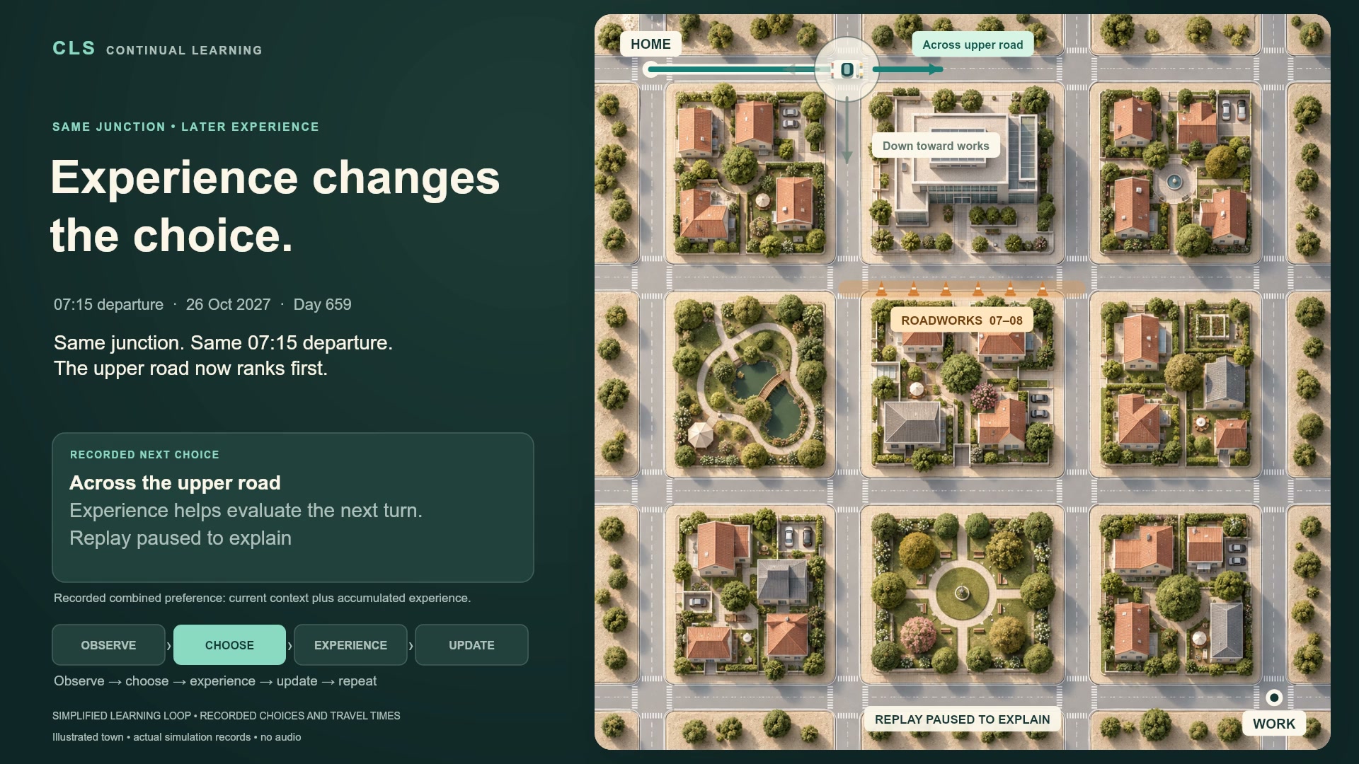
Learning while the world changes
See how Wakeline’s CLS learns from traffic delays, then learns to act on forecasts, using learning mechanisms carried across domains.
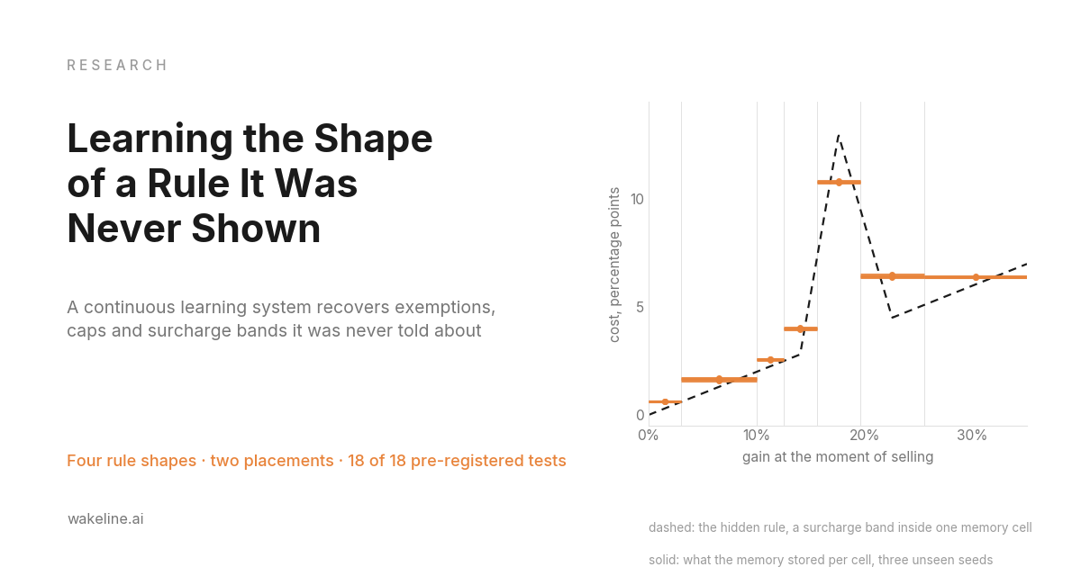
Learning the Shape of a Rule It Was Never Shown
A continuous learning system recovers hidden cost rules from the consequences of its own decisions, revealing the shape of an exemption, a cap, a surcharge band and a progressive kink.
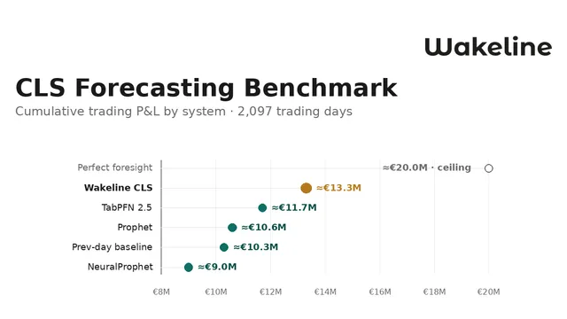
The CLS Forecasting Benchmark: Continual Learning Measured in Euros
The CLS forecasting function delivers approximately 14% higher cumulative trading P&L than TabPFN over 2,097 trading days on the German-Luxembourg day-ahead market. We present the benchmark results, methodology and limitations.

Investment Opportunities
We are currently engaging with investors and strategic partners interested in long-term technological impact grounded in scientific discipline.
Wakeline represents a fundamentally different approach to artificial intelligence, prioritizing continuous adaptation, reduced compute dependence, and real industrial application.
Conversations focus on collaboration, evidence building, and shared ambition.